
How to prepare a protein model for aptamer design
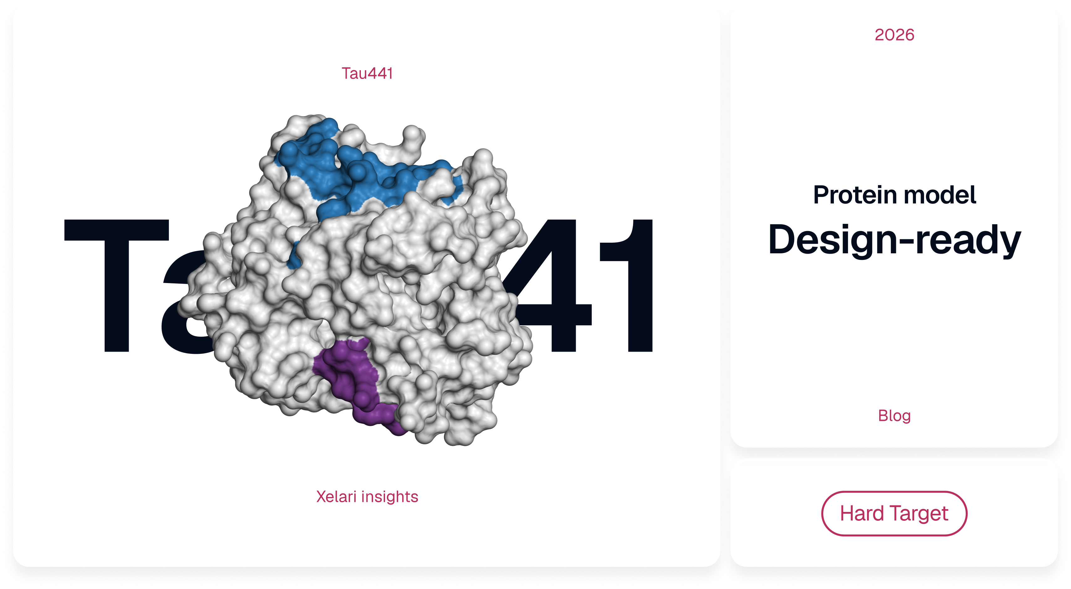
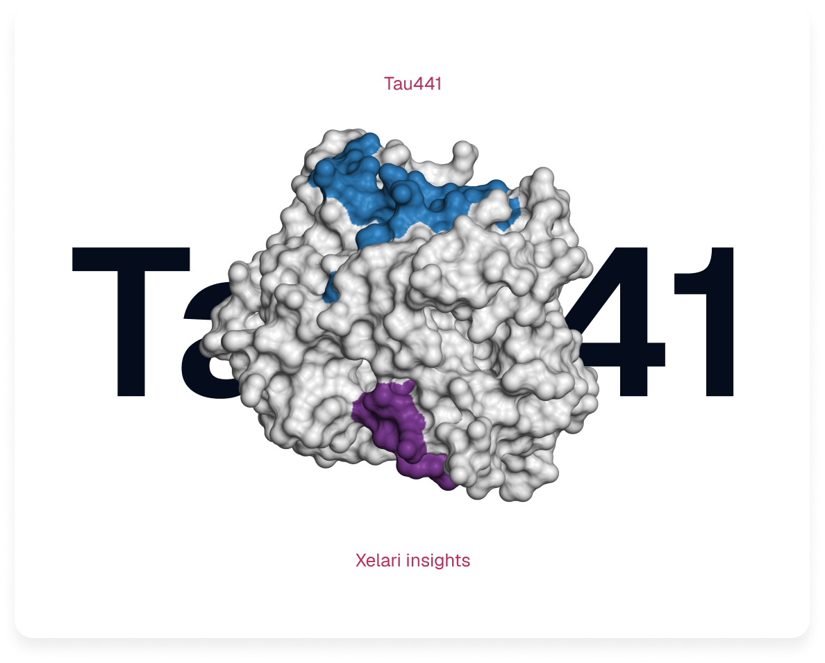
A practical guide for difficult targets, with human Tau441 as a worked example
A protein model can look finished on screen and still lead an aptamer design in the wrong direction. The file may represent another isoform, omit the modification your assay depends on, or show a binding surface that disappears when the target joins its natural complex. A complete chain and an attractive 3D picture do not protect against those errors.
You do not have to be a structural bioinformatician to notice many of these problems. What matters is knowing what the coordinates describe, which parts are supported by evidence and which questions must be answered experimentally. This guide is written for molecular biologists, assay developers and researchers who commission or use structure-guided aptamer design.
This is the next step after Xelari's How to choose the right binding site for your aptamer. That article explains how to choose a fragment to search and an anchor point to guide design. Here, we start with that provisional choice and ask a different question: which structural coordinates can support it and what needs to be checked before using them? If you have not chosen the region yet, start with the site-selection article.
Preparation does not aim at the most complete-looking model. It aims at coordinates that represent a plausible, reachable binding region in the molecular state your assay will actually meet.
Three questions before you open the file
An aptamer is a short DNA or RNA molecule that folds into a three-dimensional shape and binds a target. Its binding region (often called an epitope) is not merely a residue number: the aptamer must make physical contact with an area of protein surface. A PDB or mmCIF coordinate file contains one structural representation of that area; it does not guarantee that the representation is the state present in your sample.
Before starting, ask whether the file describes the right molecule, whether the local geometry at the proposed site has credible evidence and whether a folded aptamer can reach the surface. A sandwich assay adds a fourth practical consideration: the antibody or other detection reagent also needs room on the same target.
These questions lead to seven steps. You may move through them quickly when an experimental structure is available, or return to earlier steps when a flexible, modified, or poorly characterized protein needs alternatives.
I. The preparation path
Step 01. Define the molecule the aptamer will meet
Tools: UniProt, the exact construct sequence, the supplier's certificate of analysis and the assay protocol.
Typical time: 30-60 minutes when sample documentation is available.
A protein name is not a specification. "Human tau" might refer to several splice isoforms, a fragment released by proteolysis, or a phosphorylated molecular species. The structural consequences are immediate: the same surface may be exposed in a soluble monomer, hidden at an oligomer interface, or absent from a circulating fragment.
Start with the species, accession and isoform, then obtain the amino-acid sequence of the material actually used. Save it as a FASTA file–a plain-text sequence with a header–because it gives the project a reference for residue numbering. Record construct boundaries, engineered substitutions, purification tags and cleavage sites. A residue numbered 390 in the reference protein is not necessarily numbered 390 in a fragment or a different isoform.
The protein's chemical and physical state also belongs in the brief. Note phosphorylation or glycosylation at specified positions, disulfides, relevant metal ions, partner chains and whether the protein is monomeric, aggregated, membrane-associated or immobilized. Include the assay buffer, pH, ionic composition, temperature and sample matrix. For an aptamer, magnesium is not merely a buffer detail: it can change nucleic-acid folding and binding. [1]
Finally, carry forward the chosen fragment and anchor point, keeping their biological numbering explicit. The eventual epitope is the surface contacted by the aptamer, not necessarily a single anchor residue. If an antibody must also bind, record the region it needs to reach. Revisit the site choice only when structural evidence shows it cannot meet the assay's requirements.
Before moving on: keep one reference FASTA and a documented molecular state. If the construct or modification state is unknown, ask the sample provider rather than inferring it from the first database model.
Step 02. Find out what existing structures actually resolve
Tools: RCSB PDB (primary search for experimental structures), UniProt (reference sequence), AlphaFold DB (predicted structures); PDBe-KB and SIFTS (additional residue mapping), ChimeraX or PyMOL (inspection).
Typical time: 1-3 hours for a well-studied target.
Start at RCSB PDB and search for experimental structures by UniProt accession or protein sequence. An X-ray, cryo-EM or NMR entry may already describe the region you need. Open a candidate entry, note its PDB identifier, chain, experimental method and sequence coverage and compare the modeled construct with the protein in your assay. Download the original PDBx/mmCIF coordinates rather than relying on a screenshot.
Use PDBe-KB for additional protein-centered annotations and SIFTS when you need to match PDB residue numbers to a UniProt sequence or isoform. That mapping is also used in RCSB resources; it is a check on residue identity, not on whether a predicted interface is correct.
What does the experimental structure actually contain? A deposited structure can include stabilizing mutations, missing loops, only one domain, a bound inhibitor, or a crystallographic arrangement different from the solution assembly. Inspect the intended site directly. For crystal structures, ask whether a neighboring symmetry-related molecule contacts the surface. For cryo-EM structures, local map support matters more than global resolution alone.
A short experimental fragment can sometimes be the better choice. If an experimentally resolved 70-residue domain covers the target patch and distant regions cannot plausibly reach it, adding a speculative full-length chain may increase uncertainty rather than useful information. But the fragment is not sufficient when omitted segments could cover the site or prevent a second binder from approaching.
If you only have a predicted model, look at two different confidence measures. pLDDT reports local confidence around residues, while PAE (predicted aligned error) helps assess whether separated parts of the protein are placed reliably relative to one another. Neither tells you how the target behaves in your exact buffer. [2][3] A model with a high average score may still have an uncertain loop exactly where the aptamer is supposed to bind.
Low confidence in an intrinsically disordered region can reflect genuine structural diversity rather than a broken prediction. Do not force such a segment into a neat fold merely to obtain a complete file. [2][4] An aptamer can recognize a flexible region, but one snapshot may be a poor description of its accessible states.
Before moving on: record the selected PDB ID and chain (or predicted-model source), reconcile residue numbering with the reference FASTA and mark the proposed region as experimentally resolved, template-derived, predicted or unresolved. Inspect nearby regions that might hide the patch. If evidence is weak, record the gap before modeling anything new.
Step 03. Use measurements to constrain uncertainty, without asking them to do too much
Tools: PRIDE or jPOST for cross-linking data, BMRB for NMR, SASBDB for scattering data and the relevant primary papers.
Typical time: several hours to days when suitable data exist.
When the structure does not determine the important region, experiments can narrow the possibilities. They do not all measure the same thing. Cross-linking mass spectrometry (XL-MS) provides evidence that two chemically linked residues approached within the reach of a particular reagent. It does not fix one exact backbone distance; in a flexible protein, cross-links collected from many molecules may come from different conformations. [5][6]
Nuclear magnetic resonance (NMR) can report local conformational preferences and dynamic contacts. Small-angle X-ray scattering (SAXS) provides information on overall size and shape in solution. Hydrogen–deuterium exchange mass spectrometry (HDX-MS) reports exchange and protection, which depend on solvent access, hydrogen bonding and local opening, not simply a geometric surface area. [7][8] Antibody–peptide complexes can strongly constrain the local bound geometry of an epitope without proving that it adopts the same geometry when free.
| Evidence | What it helps you judge | What it cannot prove alone |
|---|---|---|
| XL-MS | Compatible residue-pair proximity, with chemistry-dependent distance ranges. | One exact Cα–Cα distance or one conformation satisfying all links simultaneously. |
| NMR | Local structure preferences, motion and selected contacts. | A single dominant full-length fold for a dynamic chain. |
| SAXS | Solution dimensions and ensemble-averaged shape under defined conditions. | Unique atomic coordinates. |
| HDX-MS | Protection and changes in molecular dynamics or accessibility. | Static solvent exposure or an exact contact map. |
| Binder–antigen structures | Local geometry of the bound peptide or region in the observed complex. | The free protein conformation or the footprint of a different antibody. |
Evidence
XL-MS
What it helps you judge
Compatible residue-pair proximity, with chemistry-dependent distance ranges.
What it cannot prove alone
One exact Cα–Cα distance or one conformation satisfying all links simultaneously.
Evidence
NMR
What it helps you judge
Local structure preferences, motion and selected contacts.
What it cannot prove alone
A single dominant full-length fold for a dynamic chain.
Evidence
SAXS
What it helps you judge
Solution dimensions and ensemble-averaged shape under defined conditions.
What it cannot prove alone
Unique atomic coordinates.
Evidence
HDX-MS
What it helps you judge
Protection and changes in molecular dynamics or accessibility.
What it cannot prove alone
Static solvent exposure or an exact contact map.
Evidence
Binder–antigen structures
What it helps you judge
Local geometry of the bound peptide or region in the observed complex.
What it cannot prove alone
The free protein conformation or the footprint of a different antibody.
The practical rule is to keep observations separate from models already fitted to them. Agreement with a restraint used to build the model tests internal consistency; it is not an independent validation. If feasible, reserve at least one experiment as a later check. State the conditions, data identifiers, interpretation and uncertainty rather than converting every measurement into a rigid coordinate requirement. [4][9]
Before moving on: you should be able to say which experimental observations support your target geometry, which remain inconsistent and which important assumptions are still model-dependent.
Step 04. Generate alternatives only where they could change the answer
Tools: Boltz-2, Rosetta or MODELLER when appropriate; ChimeraX or PyMOL for local alignment.
Typical time: hours to days, depending on complexity and computing resources.
Not every uncertain residue needs a major simulation campaign. A stable domain may require one loop reconstruction or a comparison of plausible side-chain orientations. A disordered protein may require distinct local backbones and different long-range arrangements, especially if a distant stretch of chain could cover the chosen patch.
The useful question is not how many structures can we produce? It is which uncertain structural feature could change our design decision? Align candidates on the target region rather than on the whole chain. Then compare the shape of the proposed interface, which side chains point outward and which neighboring segments prevent approach. Do not select a model merely because it looks compact, smooth or geometrically tidy.
An especially informative sensitivity test is to remove or vary the least-supported long-range interaction that creates the binding pocket. If the pocket disappears, the design relies on an uncertain contact. That can justify carrying two plausible models into design or choosing a different surface.
Model generators produce structural hypotheses, not necessarily a physically weighted population of conformations in solution. Ten similar outputs do not mean the protein spends ten times longer in that state. Estimating solution populations requires additional evidence and methods appropriate for ensembles. [4][10][11]
Before moving on: retain a representative set of alternatives only if differences could affect binding. Otherwise document why one local representation is adequate.
Step 05. Ask whether a folded aptamer can actually reach the site
Tools: FreeSASA, Biopython's Shrake–Rupley method, ChimeraX or PyMOL for surfaces and steric inspection; APBS/PDB2PQR for optional electrostatics.
Typical time: 1-2 hours for an initial screen, more for complex docking.
A site can be present in the sequence, exposed to water and still be unreachable by an aptamer. Solvent-accessible surface area (SASA) is usually calculated with a small probe of radius 1.4 Å, approximately the size of a water molecule. A folded DNA or RNA aptamer has a far larger three-dimensional footprint and may approach from only a few directions.
Start with chemical integrity: are the atoms of the proposed surface present, along with its phosphorylation, nearby glycans and relevant neighboring chains? Then assess surface exposure, residue by residue, across the conformations that remain plausible. Relative solvent accessibility (RSA) scales SASA by a residue-specific reference maximum. Always state which normalization you used. Values can help compare surfaces, but there is no experimentally established universal RSA cutoff for declaring an aptamer site accessible. [12]
The decisive check is physical approach. Inspect the area around the patch, not just the patch itself. Could the entire folded aptamer reach it without colliding with another domain, a glycan, a membrane or an immobilization surface? If an aptamer structure or docking pose is available, examine the complex; do not infer binder clearance from the protein alone. Nearby electrostatic surfaces and the assay's salt composition can change the plausibility of a pose even when there are no obvious steric clashes.
Sandwich assays introduce a second footprint. Two sites far apart in sequence can be adjacent in 3D, while a nominal gap between their Cα atoms says little about the space required by a folded aptamer and an antibody Fab. Model both binders if possible, then verify simultaneous function experimentally. Immobilization adds another constraint: a surface exposed in solution can face the membrane or bead after attachment.
Before moving on: record which surfaces appear exposed, which states could block them and whether a real binder approach has been evaluated or remains a hypothesis.
Step 06. Repair the chemistry; relax only when it buys something
Tools: PDBFixer and pdb-tools for supported coordinate repairs; Reduce and appropriate pH/protonation tools; GROMACS, OpenMM or Amber only when relaxation is justified.
Typical time: 1–3 hours for a simple repair; much longer for parameterization or MD.
A selected model may still have missing atoms, broken segments, incorrect terminal groups, wrong protonation assumptions, alternate atom positions or chain-numbering changes. Check the structure against the same reference FASTA used at the start. Inspect disulfide bonds, covalent labels, cofactors, metals, glycans and partner chains that belong in the experimental target state.
In legacy PDB files, nonstandard molecules can appear as HETATM records. Deleting every HETATM entry is not a cleanup strategy: it can discard a required metal, cofactor, glycan or ligand. Modified amino acids also need special attention. Phosphothreonine and phosphoserine may be identified by the chemical component codes TPO and SEP, but correct atom labels do not guarantee that a downstream program retains them during import. Test the final imported file, not only the export.
Energy minimization can remove severe local strain. Short molecular dynamics (MD) can allow immediate structural relaxation and identify obvious local instability. Neither operation validates a predicted fold or generates an equilibrium ensemble of a disordered protein. If phosphorylated residues are included, ensure that the simulation uses compatible parameters. [13] Compare the geometry, experimental restraints and binding-site exposure before and after relaxation. A lower calculated energy is not a biological validation.
Before moving on: save the prepared coordinates plus a record of every repair and relevant assumption. If a repair moves the site or changes the target's molecular state, reconsider the candidate rather than accepting the altered model automatically.
Step 07. Audit the exact file you are sending
Tools: MolProbity for all-atom geometry, Gemmi or Biopython for sequence/site screening.
Typical time: 15–60 minutes for an uncomplicated file, excluding repairs.
The most important handoff rule is simple: reopen the exported file in the software that will actually use it. Check the chain IDs, numbering, modified residues, atom completeness and import warnings. A modification that disappears during conversion can change the recognition problem even when the source PDB looked correct.
Separate two kinds of quality control. A fast identity and site screen aligns the coordinate sequence with the reference FASTA, identifies missing positions and substitutions, checks the specified PTM labels and records exposure and geometric dimensions. An all-atom validation examines steric overlaps using atom-specific van der Waals radii, backbone and side-chain geometry, chirality and unusual peptide bonds. A generic fixed distance threshold is not a replacement for MolProbity. [14] Rare nonproline cis-peptide bonds deserve investigation; they are not automatically chemically impossible.
For flexible proteins, record the model's radius of gyration (Rg), which measures how spread out the coordinates are. Compare it with relevant solution experiments and with other plausible conformations, not blindly with an ideal globular-protein formula. The Cα-based Rg of one coordinate file is not identical to an ensemble-averaged experimental SAXS quantity. Note which atoms and weighting method were used.
The deliverable is more than a PDB or mmCIF. It is the coordinate file plus its preparation record: reference sequence, molecular state, source structures, evidence and modeling decisions, software versions, geometry review, remaining uncertainty and, ideally, file checksums. You can ask a structural specialist to produce this record even if you do not personally run every program.
Before moving on: you should be able to give the file to a collaborator without requiring them to guess what it contains, why it was chosen or what it cannot establish.
The short route for a well-resolved protein
Not every target needs Boltz, a conformational ensemble or molecular dynamics. When a good experimental structure covers the right molecular state and the intended patch, the workflow can be brief.
Align its coordinate sequence to the reference FASTA
Inspect local experimental support and biologically relevant neighboring chains
Check the intended approach
Repair only what is necessary
Validate geometry and reopen the export.
If each check is satisfactory, stop. Extra modeling can add unsupported assumptions to a problem that was already solvable.
II. Tau441 in practice: the seven steps applied
Case sources: human Tau441 (UniProt P10636-8); PDB 6XLI, 5E2W and 5E2V; Popov XL-MS data (PRIDE PXD015044); Boltz-2; GROMACS.
Our Tau441 project began with a concrete assay requirement. The capture DNA aptamer was to recognize a region near Ala390; an antibody reporter associated with phosphorylated Thr217 also needed access to the same protein. [15] Those two sites are far apart in sequence, but Tau441 is highly flexible in solution, so the shape of the chain can affect whether either site is presented to a binder.
The seven steps below follow Part I in the same order. We built the Tau441 model for our aptamer-design project and described the workflow in our research publication. [15] Here, we revisit those modeling decisions alongside the final Tau441 structure.
Step 01. Define the molecule the aptamer will meet
Tau441 evidence and tools: UniProt P10636-8; human 2N4R tau; phosphorylated residues; Ala390 and pThr217 assay requirements.
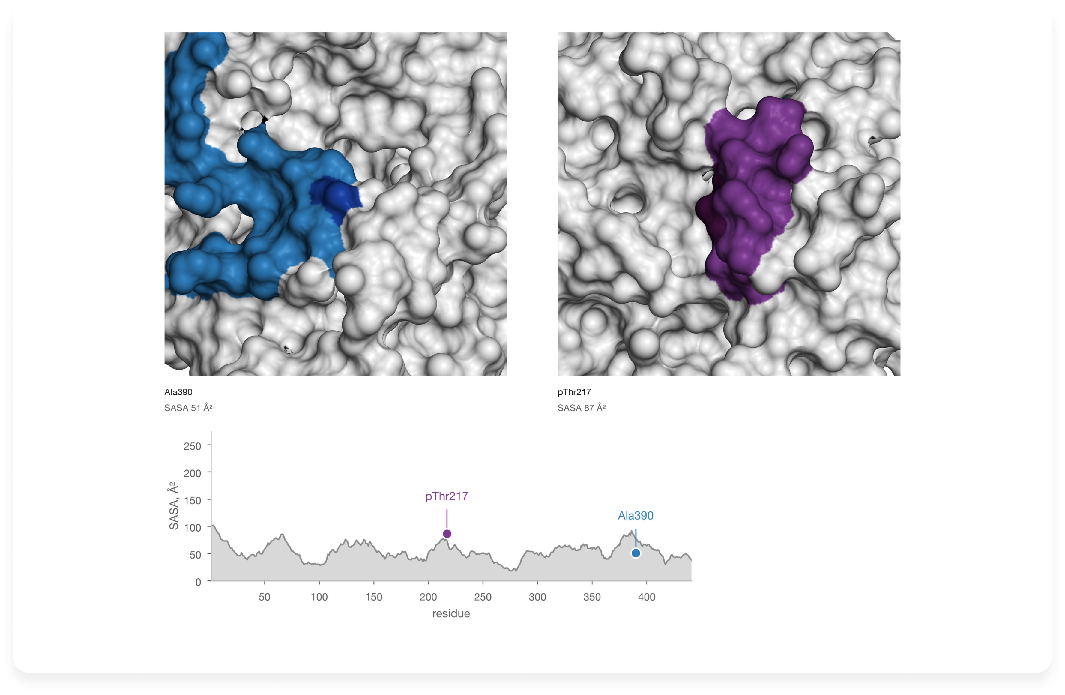
We chose the full-length human 2N4R isoform - 441 amino acids, UniProt P10636-8 as the numbering reference. The design brief specified an aptamer target centered on Ala390 and an antibody-associated region around pThr217. The proposed aptamer interface was later placed near residues 380-400 by the design and docking results. [15] These positions gave us two named regions to track from the initial sequence through the final structure.
The model was prepared with seven phosphorylated positions: Thr181, Ser202, Thr205, Ser208, Thr212, Thr217 and Thr231. Defining these sites in advance ensured that the phosphorylation-sensitive antibody region would be modeled with the intended chemistry.
A fragment containing only Ala390 would be easier to handle, but it would omit distant tau segments capable of crossing that surface–and the separate antibody-associated region. We therefore worked with the full chain. At the end of this first step, the project had an explicit sequence, modification pattern and two-site design requirement. Those became the reference against which the available structures were judged.
Step 02. Find out what existing structures actually resolve
Tau441 evidence and tools: RCSB PDB 6XLI and 5E2W as the reported local templates; 5E2V for comparison; full-length NMR and filament structures for molecular-state context.
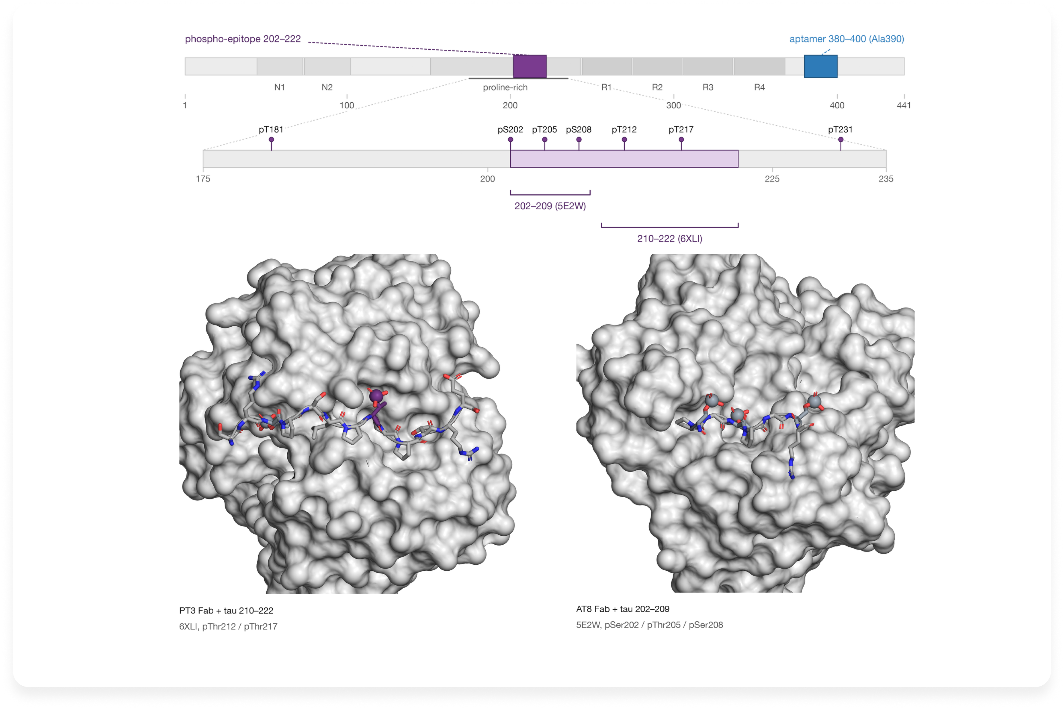
RCSB PDB did not contain an experimentally resolved, full-length soluble Tau441 conformation suitable for this assay. It did contain short, highly informative antibody-bound peptides. In 6XLI, the PT3 Fab binds a tau peptide phosphorylated at Thr212 and Thr217. In 5E2W, AT8 binds a peptide phosphorylated at Ser202, Thr205 and Ser208; its related structure 5E2V contains the first two phosphates without pSer208. [16][17] The published modeling used 6XLI and 5E2W to guide local phosphoepitope geometry.
These crystal structures supplied coordinates for short regions, not the position of those regions within the whole soluble tau chain. They also depict PT3 and AT8, whereas the assay used a different, proprietary 3-H antibody. We used the observed peptide conformations as local structural evidence without assuming that the antibody footprints were interchangeable. Solution NMR provided context for tau’s conformational variability; [7] the ordered core seen in Alzheimer-associated filaments belongs to an aggregated molecular state. [18]
Readers can see the distinction directly in the RCSB 3D viewer: open 6XLI, locate the tau phosphopeptide among the antibody chains and identify the two phosphorylated threonines. Then compare the bound tau peptides in 5E2V and 5E2W to see where pSer208 changes the chemical state. Mapping these short peptide sequences back to 2N4R numbering is the practical link between experimental fragments and the full-length model. The resulting template map covered useful short segments while leaving the global arrangement to be modeled.
1. Structural evidence
Step 03. Use measurements to constrain uncertainty, without asking them to do too much
Tau441 evidence and tools: XL-MS and chemical surface-labeling evidence; PRIDE dataset PXD015044
The peptide structures answered a local question: how might these phosphorylated stretches be shaped when recognized? To examine how more distant parts of the chain could be arranged, the study drew on Popov and colleagues’ structural-proteomics evidence, including 118 short-range cross-links and surface-modification measurements. [5][15] The cross-links contributed information about residue pairs that had approached one another, while the surface measurements helped assess which stretches could be exposed.
The prior Popov model placed the Thr212/Thr217 region in a relatively inaccessible environment for the intended antibody-based assay. [5][15] This motivated a search for other conformations that could accommodate the experimental observations while presenting that region more openly. In the reported Boltz-2 modeling, the cross-links acted as soft distance guidance: their role was to favor compatible arrangements, rather than freeze the flexible chain into one set of exact distances.
Step 04. Generate alternatives only where they could change the answer
Tau441 evidence and tools: Boltz-2; full-length sequence, specified phosphorylation, local peptide templates and XL-MS-derived restraints
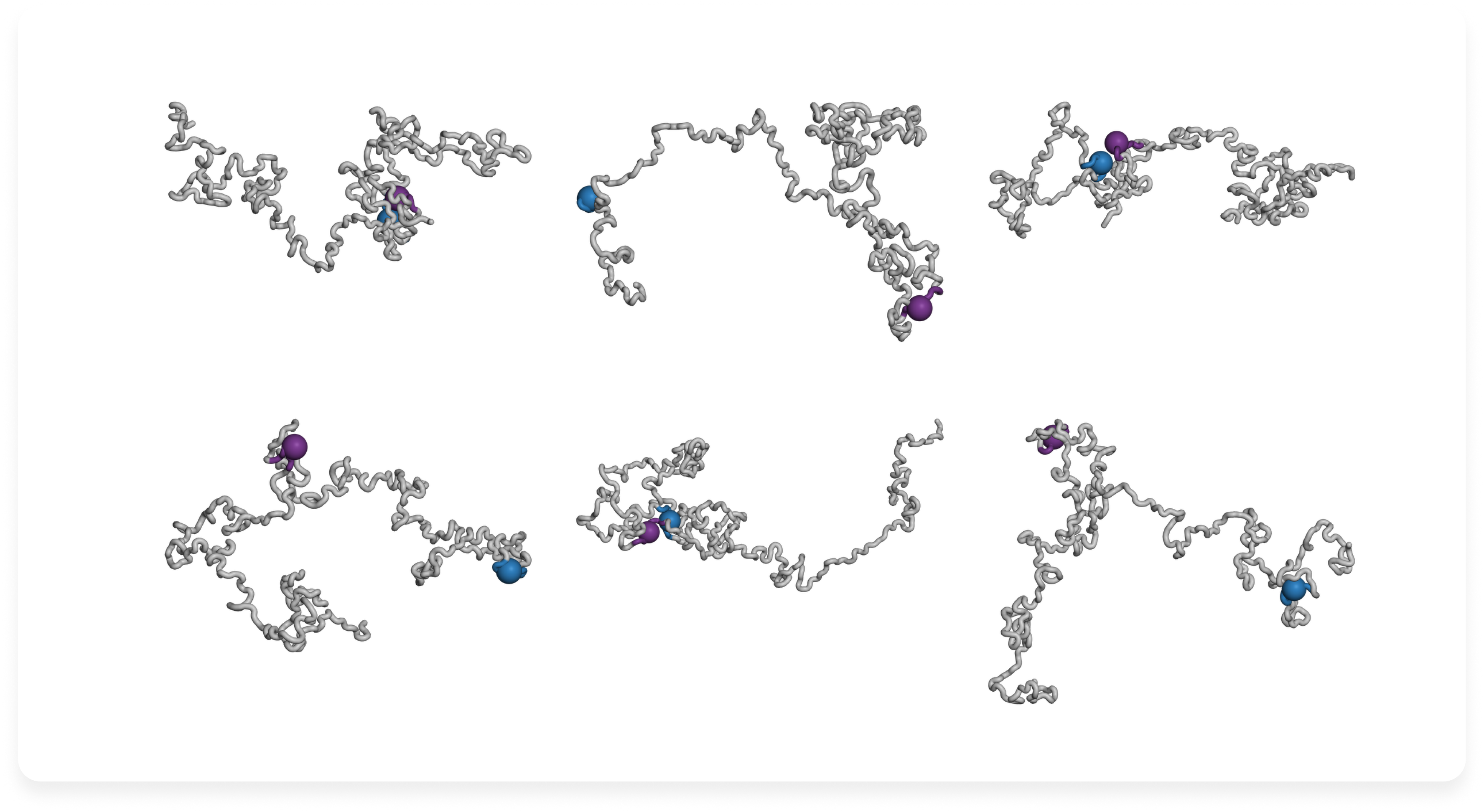
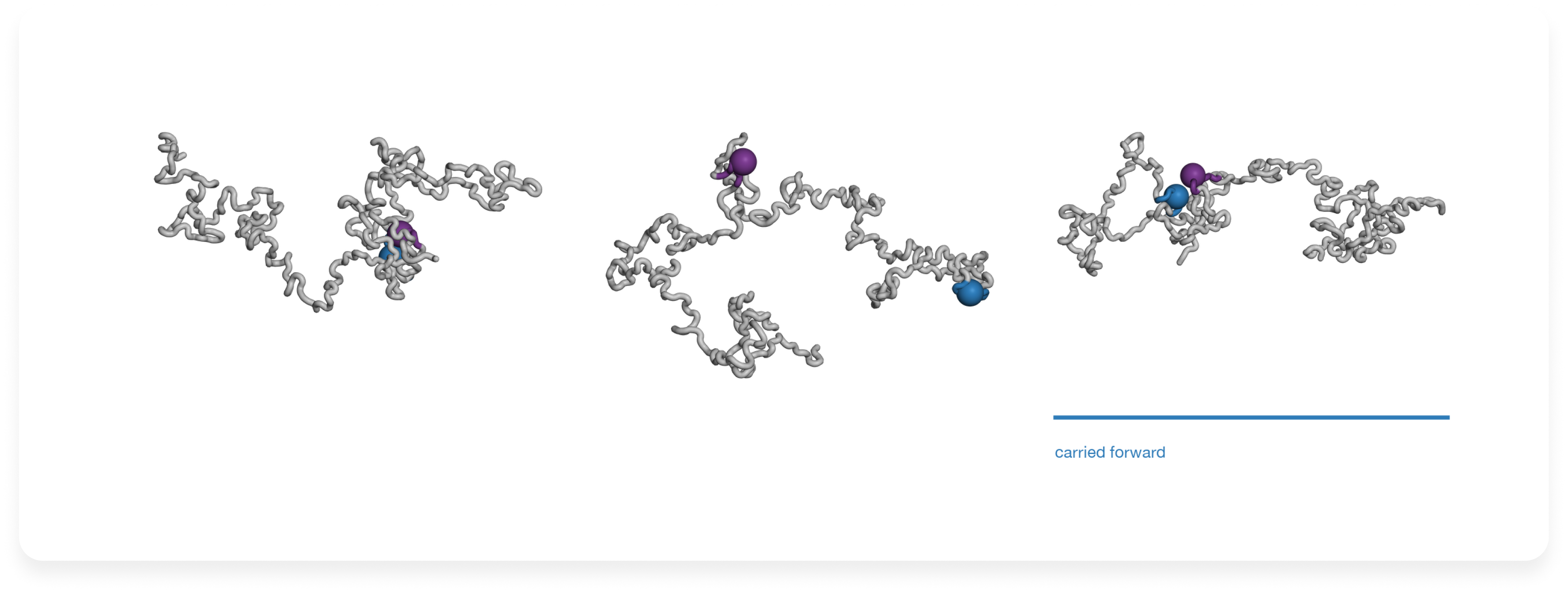
We generated full-length candidate structures with Boltz-2, combining the 441-residue sequence and modified sites with local template information and the XL-MS constraints. We subsequently reported dozens of independent diffusion samples and roughly 10-15 recycling cycles. [15] Independent runs can produce different chain arrangements; recycling revisits a candidate during prediction. This sampling was useful because the relative placement of distant tau segments is less securely known than the short experimental peptide geometries.
For Tau441, a coherent input description had to preserve the same 2N4R residue numbering across the sequence, the seven modifications, the peptide templates and the cross-link pairs. Our publication describes these inputs and the sampling strategy.
2. Conformational sampling
Step 05. Ask whether a folded aptamer can actually reach the site
Tau441 evidence and tools: SASA screening of phosphoepitopes; local backbone comparison with 6XLI/5E2W; inspection of the two assay regions
We evaluated the Boltz-2 candidates against three criteria: exposure of pThr217 and other antibody-associated phosphoepitopes, local backbone agreement with the experimental peptide templates and absence of obvious global collapse. [15] Keeping the pThr217 region accessible was important for the reporter antibody. Near Ala390, the full-length models supplied the surrounding chain context for subsequent aptamer design.
We further modeled the Tau181-235 segment using PDB 6XLI as a local template. The reported backbone RMSD of 0.71 Å describes agreement with that template in the local comparison. [15][16] On the basis of the selection criteria, we chose one working conformation for the subsequent MD relaxation.
3. Candidate selection
Step 06. Repair the chemistry; relax only when it buys something
Tau441 evidence and tools: GROMACS 2024.1; Amber ff19SB with phosphorylation-compatible parameters; OPC3 water; 10 ns simulation
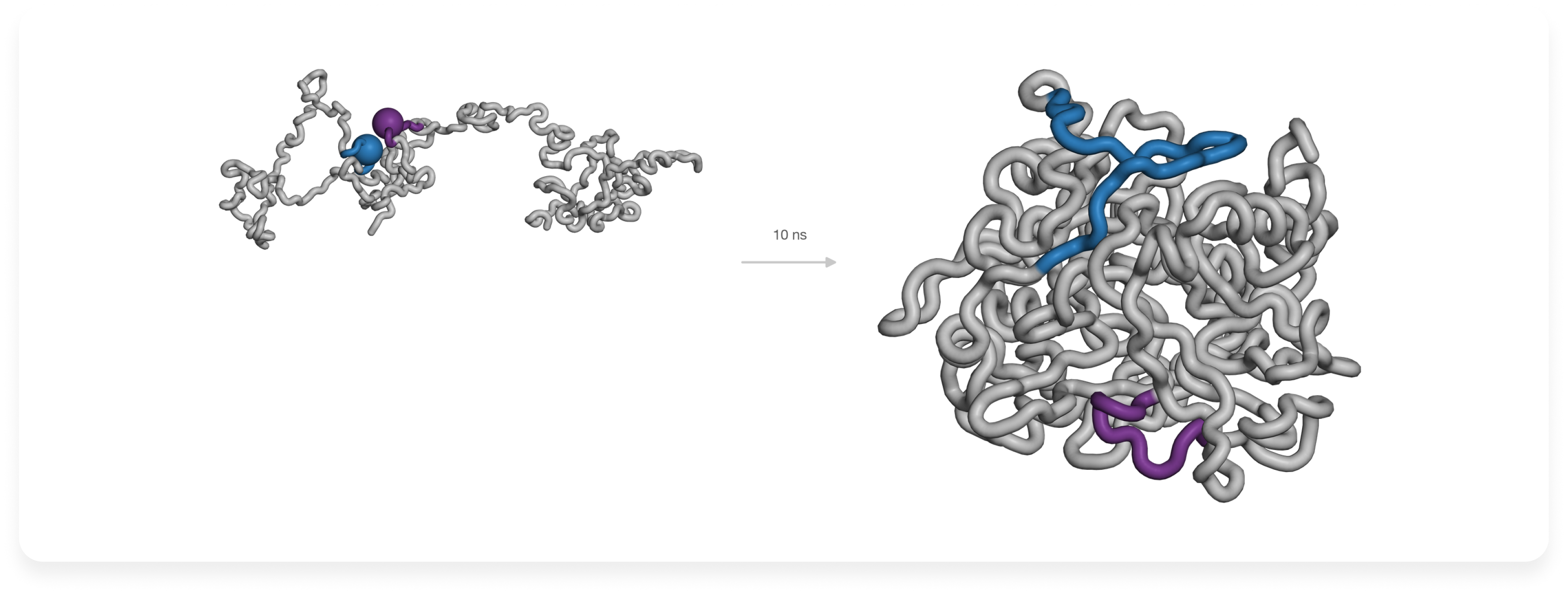
After selecting a candidate, we relaxed its coordinates by molecular dynamics. The protocol used 10 ns in GROMACS 2024.1 with Amber ff19SB, dedicated parameters for phosphorylated amino acids and explicit OPC3 water. [13][15] The selected tau representation carried seven phosphate groups, so ordinary unmodified-serine and unmodified-threonine parameters would not represent the intended system.
The purpose of this short run was local adjustment of the chosen structure before aptamer design, rather than exhaustive sampling of all Tau441 conformations. It produced a trajectory from which a representative coordinate set could be selected. For this Tau441 input, a reproducible follow-up would compare the neighborhoods of Ala390 and pThr217 before and after the run and confirm the seven modified residue chemistries remain supported. The main simulation settings are reported. [15]
4. Molecular dynamics refinement
Step 07. Audit the exact file you are sending
Tau441 evidence and tools: Trajectory clustering; Xelari aptamer-design platform.
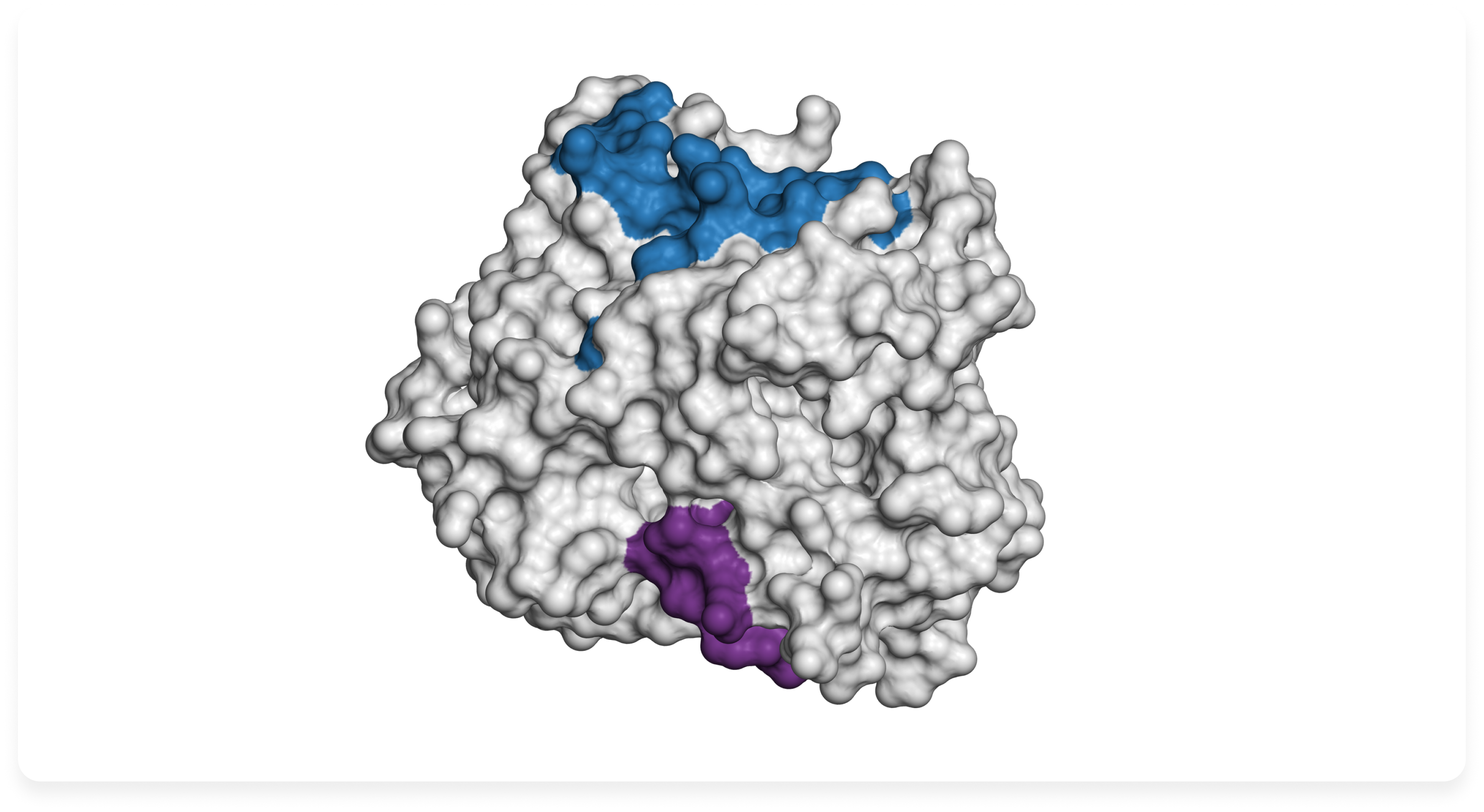
Following the 10 ns molecular dynamics relaxation, we grouped similar snapshots from the trajectory using a 0.25 nm clustering cutoff. We selected the centroid of the most populated cluster as the final protein structure. [15] This gave us a representative coordinate set from the relaxed Boltz-2 candidate, ready for use in aptamer design.
The prepared model contained the full 441-residue Tau chain, including seven modeled phosphorylation sites: Thr181, Ser202, Thr205, Ser208, Thr212, Thr217 and Thr231. We used this structure as the input for aptamer design on the Xelari platform, targeting the region around Ala390 while keeping the antibody-associated pThr217 region in mind. The subsequent design stage produced a proposed aptamer-binding arrangement involving approximately residues 380-400. [15]
The aptamer-design conditions were specified separately from the protein relaxation protocol: 25 °C, pH 7.2, 137 mM Na⁺, 2.7 mM K⁺ and no Mg²⁺. [15] These conditions matter because the folding and binding behavior of a DNA aptamer can change with temperature, pH and ionic composition. We discuss these effects in more detail in our companion article, Why pH, Temperature and Ions Belong in the Design Specification.
For a similar project, the final handoff should include the exact protein coordinates and a short preparation record documenting the reference sequence, modeled modifications, experimental templates, structural constraints and refinement method. Before starting design, confirm that the receiving software correctly interprets residue numbering and phosphorylated amino acids. This ensures that the binding region selected earlier in the workflow is the same region used for aptamer design.
5. Final Tau441 model
6. Binding-site inspection
The best model is not the one with the most coordinates. It is the least speculative representation that keeps the chemistry and the access you need in order to ask the next experimental question.
References and further reading
- Kohlberger M, Gadermaier G. SELEX: critical factors and optimization strategies for successful aptamer selection. Biotechnology and Applied Biochemistry. 2022;69:1771–1792. doi:10.1002/bab.2244.
- Alderson TR, Pritišanac I, Kolarić D, Moses AM, Forman-Kay JD. Systematic identification of conditionally folded intrinsically disordered regions by AlphaFold2. PNAS. 2023;120:e2304302120. doi:10.1073/pnas.2304302120.
- Abramson J, Adler J, Dunger J, et al. Accurate structure prediction of biomolecular interactions with AlphaFold 3. Nature. 2024;630:493–500. doi:10.1038/s41586-024-07487-w.
- Borthakur K, Sisk TR, Panei FP, Bonomi M, Robustelli P. Determining accurate conformational ensembles of intrinsically disordered proteins at atomic resolution. Nature Communications. 2025;16:9036. doi:10.1038/s41467-025-64098-3.
- Popov KI, Makepeace KAT, Petrotchenko EV, Dokholyan NV, Borchers CH. Insight into the structure of the "unstructured" tau protein. Structure. 2019;27:1710–1715.e4. PRIDE PXD015044. doi:10.1016/j.str.2019.09.003.
- Bartolec TK, Vázquez-Campos X, Norman A, et al. Cross-linking mass spectrometry discovers, evaluates and corroborates structures and protein–protein interactions in the human cell. PNAS. 2023;120:e2219418120. doi:10.1073/pnas.2219418120.
- Mukrasch MD, Bibow S, Korukottu J, et al. Structural polymorphism of 441-residue tau at single residue resolution. PLOS Biology. 2009;7:e1000034. doi:10.1371/journal.pbio.1000034.
- Bradshaw RT, Marinelli F, Faraldo-Gómez JD, Forrest LR. Interpretation of HDX data by maximum-entropy reweighting of simulated structural ensembles. Biophysical Journal. 2020;118:1649–1664. doi:10.1016/j.bpj.2020.02.005.
- Vallat B, Webb BM, Zalevsky A, et al. PDB-IHM: a system for deposition, curation, validation and dissemination of integrative structures. Journal of Molecular Biology. 2025;437:168963. doi:10.1016/j.jmb.2025.168963.
- Tesei G, Trolle AI, Jonsson N, et al. Conformational ensembles of the human intrinsically disordered proteome. Nature. 2024;626:897–904. doi:10.1038/s41586-023-07004-5.
- Jeon J, Yang W, Park S, Kim JH, Lee Y-H, Yu W. Accurate conformational ensembles of intrinsically disordered proteins using reweighting based on NMR chemical shifts. PNAS. 2026;123:e2518125123. doi:10.1073/pnas.2518125123.
- Tien MZ, Meyer AG, Sydykova DK, Spielman SJ, Wilke CO. Maximum allowed solvent accessibilities of residues in proteins. PLOS ONE. 2013;8:e80635. doi:10.1371/journal.pone.0080635.
- Raguette LE, Cuomo AE, Belfon KAA, et al. phosaa14SB and phosaa19SB: updated Amber force field parameters for phosphorylated amino acids. Journal of Chemical Theory and Computation. 2024;20:7199–7209. doi:10.1021/acs.jctc.4c00732.
- Williams CJ, Headd JJ, Moriarty NW, et al. MolProbity: more and better reference data for improved all-atom structure validation. Protein Science. 2018;27:293–315. doi:10.1002/pro.3330.
- Mahrat R, Chen Y, Bruno JG, Nasaev S, Ufaev D, Kudryashova N. Preliminary development of a hybrid aptamer and antibody fluorescent lateral flow assay for ultrasensitive detection of Tau441 protein in serum: toward point-of-care diagnostics for Alzheimer's disease. Journal of Fluorescence. 2026. doi:10.1007/s10895-026-04925-y.
- Van Kolen K, Malia TJ, Theunis C, et al. Discovery and functional characterization of hPT3, a humanized anti-phospho tau selective monoclonal antibody. Journal of Alzheimer's Disease. 2020;77:1397–1416. PDB 6XLI. doi:10.3233/JAD-200544.
- Malia TJ, Teplyakov A, Ernst R, et al. Epitope mapping and structural basis for the recognition of phosphorylated tau by the anti-tau antibody AT8. Proteins. 2016;84:427–434. PDB 5E2W/5E2V. doi:10.1002/prot.24988.
- Fitzpatrick AWP, Falcon B, He S, et al. Cryo-EM structures of tau filaments from Alzheimer's disease. Nature. 2017;547:185–190. doi:10.1038/nature23002.
© 2026 Xelari Inc. All rights reserved.
